Core-Collapse Examples
Getting Started
Read in a lightcurve and the filename of an SED:
from __future__ import print_function
import snsedextend
sedFile=snsedextend.example_sed
myLC=snsedextend.load_example_lc()
print(myLC)
Out:
name  band     time     mag   magerr
------ ---- ----------- ------ ------
2006aj    U 53788.16733 18.039  0.078
2006aj    U 53790.12301 17.995  0.047
2006aj    U 53790.13652 17.982  0.057
2006aj    U 53796.11875 18.599  0.112
2006aj    U 53797.11978 18.679  0.054
2006aj    U 53798.16206 18.738  0.058
2006aj    B 53788.11683 18.438   0.05
...  ...         ...    ...    ...
2006aj    H    53793.12 16.752  0.047
2006aj    H   53798.145 16.635  0.037
2006aj    K    53788.16 17.183   0.12
2006aj    K   53790.133 16.714  0.094
2006aj    K   53792.123 16.406  0.145
2006aj    K    53793.12 16.393   0.08
2006aj    K   53798.145 16.769   0.08
Length = 105 rows
Generate a Color Table
Produce a color table from the example data with some assumptions. You can set any parameter that you would like that is used for SNCosmo fitting.
colorTable=snsedextend.curveToColor(myLC,colors=['U-B', 'r-J', 'r-H', 'r-K'],snName='testSN',
                 snType='Ic', zpsys='vega', bounds={'hostebv': (-1, 1),
                 't0': (53787.94, 53797.94)},constants={'mwr_v': 3.1,
                 'mwebv': '0.1267', 'z': '0.033529863', 'hostr_v': 3.1},
                 dust='CCM89Dust', effect_frames=['rest', 'obs'], effect_names=['host', 'mw'])
Out:
Getting best fit for: U-B,r-J,r-H,r-K
No model provided, running series of models.
Best fit model is "snana-2004fe", with a Chi-squared of 310.573042
Now print the result:
print(colorTable)
Out:
        time                U-B                UB_err       ...        r-K                rK_err         SN
      float64             float64             float64       ...      float64             float64        str6
------------------- ------------------- ------------------- ... ------------------ ------------------- ------
 -4.350285244130646                  --                  -- ... 0.8720948404717248 0.14190154120165033 testSN
 -4.350285244130646                  --                  -- ...                 --                  -- testSN
 -4.350285244130646                  --                  -- ...                 --                  -- testSN
 -4.342955244137556 -0.4295303770959613 0.11018996012483721 ...                 --                  -- testSN
-2.3872752441311604 -0.1810379007836005  0.0791907192658557 ...                 --                  -- testSN
-2.3772852441325085                  --                  -- ...                 --                  -- testSN
-2.3772852441325085                  --                  -- ... 1.0478962751844385 0.11573043046828127 testSN
                ...                 ...                 ... ...                ...                 ...    ...
  0.609714755868481                  --                  -- ...                 --                  -- testSN
  3.608464755867317  0.3375874442802953 0.14704748243950216 ...                 --                  -- testSN
  4.609494755866763 0.27337763462687903 0.08918839424997288 ...                 --                  -- testSN
   5.63471475586266                  --                  -- ...                 --                  -- testSN
   5.63471475586266                  --                  -- ...                 --                  -- testSN
   5.63471475586266                  --                  -- ... 0.7367464624686129 0.10422322617626094 testSN
  5.651774755868246 0.16543738997823354 0.09323158169391926 ...                 --                  -- testSN
Color Curve Fitting
Now we can fit this color table and get a best model by minimizing BIC. This function returns a python dictionary with colors as keys and an astropy Table object with time and color vectors as values:
curveDict=snsedextend.fitColorCurve(colorTable)
Out:
Running BIC for color:
     U-B
     r-J
     r-H
     r-K
SED Extrapolation
Now you can provide an SED to be extrapolated, and let it do the work (This is a type Ic). This will return an sncosmo.Source object and simultanously save the new SED to a file defined by newFileLoc (default current directory).:
newSED=snsedextend.extendCC(colorTable,curveDict,sedlist=[sedFile],zpsys='vega',showplots=False,verbose=True)
Plotting from Timeseries
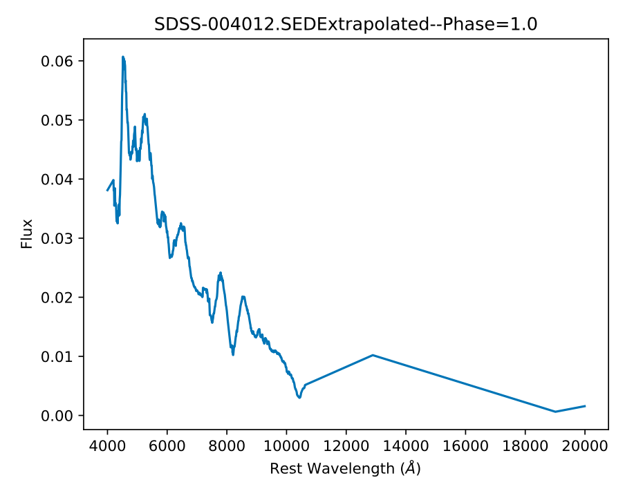
You can directly plot an SED file.:
snsedextend.plotSED('SEDS/typeIc/SDSS-004012.SED',day=1,showPlot=True,MINWAVE=4000,MAXWAVE=20000,saveFig=False)
Out: